All the math I learned from DMFT

I learned so much new math going over this tutorial on dynamical mean-field theory (DMFT) (not to be confused with DtMF). Here, I’ll try my best to document what I learned.

Linear Dynamical System with GOE Matrix

The setup is as follows:

$$\frac{d}{dt}\mathbf{h}(t)=-M\mathbf{h}(t)+\mathbf{j}(t)$$

where $\mathbf{h},\mathbf{j}\in {\mathbb{R}}^N$ and the matrix $M\in {\mathbb{R}}^{N\times N}$ is a symmetric Gaussian (GOE/Wigner) matrix: $M=\frac{1}{\sqrt{N}}A$ where $A=A^{\top }$ and $A_{ij}\sim \mathcal{N}(0,1)$. Perhaps in another note, we’ll see how the same techniques used to analyze this system can be applied to a neural network. For now, with this setup, we’ll learn and apply some fancy math (functional derivatives and Taylor expansions, the cavity method, Gaussian processes, Fourier transforms, and a little bit of random matrix theory) to informally derive Wigner’s semicircle law.

Intuition for the system we’re modeling

The way to think about the system that the above differential equation is modeling is as a time evolving network of sites $\mathbf{h}$, interconnected and interacting according to the matrix $M$, under some external influence $\mathbf{j}$ (hereon called the source). Without any external influence (i.e., $\mathbf{j}(t)=0$), the sites undergo a somewhat boring evolution described in the next section.

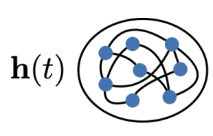
The value of a specific site $h_k(t)$ (at a specific time $t$) not only affects every other site as time moves forward, the signal propagates throughout the network and eventually returns to affect the value of $h_k(t^{\prime })$ at some later time $t^{\prime }>t$. The insight in the DMFT derivation below is that as the number of sites goes to infinity, $N\to \infty$, the distinct sites become statistically equivalent through central limit theorem (CLT)-style arguments.

Power iteration

This mini-section is somewhat irrelevant to the actual DMFT, but it’s a useful exercise to think about what happens when $\mathbf{j}(t)=0$. When $\mathbf{j}(t)=0$, the differential equation becomes $\frac{d}{dt}\mathbf{h}(t)=-M\mathbf{h}(t)$. The solution is simply an exponential:

$$\mathbf{h}(t)=e^{-Mt}\mathbf{h}(0)=e^{-U\Sigma U^{\top }t}\mathbf{h}(0)=U{e}^{-\Sigma t}{U}^{\top }\mathbf{h}(0)$$

Redefining variables such that $\tilde{\mathbf{h}}(t)=U^{\top }\mathbf{h}(t)$, we see that

$$(\tilde{\mathbf{h}}(t){)}_k=e^{-{\lambda }_{k}t}(\tilde{\mathbf{h}}(0){)}_k⟹\frac{\tilde{\mathbf{h}}(t)}{|\tilde{\mathbf{h}}(t)|}\to {\mathbf{e}}_N⟹\frac{\mathbf{h}(t)}{|\mathbf{h}(t)|}\to {\mathbf{u}}_{\min }$$

where ${\mathbf{u}}_{\min }$ is the eigenvector of $M$ corresponding to the minimum eigenvalue. This is essentially the continuous version of power iteration.

Towards a self-consistent equation

We start by manipulating the original differential equation to get an integral. Start by multiplying $e^{Mt}$ to both sides of the equation and cleverly applying the product rule.

$$e^{Mt}(\frac{d}{dt}\mathbf{h}(t)+M\mathbf{h}(t))=e^{Mt}\mathbf{j}(t)⟹\frac{d}{dt}[e^{Mt}\mathbf{h}(t)]=e^{Mt}\mathbf{j}(t).$$

Applying the fundamental theorem of calculus,

$$e^{Mt}\mathbf{h}(t)-\mathbf{h}(0)={\int }_0^t{e}^{M{t}^{\prime }}\mathbf{j}(t^{\prime })d{t}^{\prime }.$$

Finally, some algebra gets us to the form we want:

$$\mathbf{h}(t)=e^{-Mt}\mathbf{h}(0)+{\int }_0^t{e}^{-M(t-t^{\prime })}\mathbf{j}(t^{\prime })d{t}^{\prime }=e^{-Mt}\mathbf{h}(0)+{\int }_0^{\infty }{e}^{-M(t-t^{\prime })}\mathbf{j}(t^{\prime })\Theta (t-t^{\prime })d{t}^{\prime }$$

where $\Theta (t-t^{\prime })=1$ if $t>t^{\prime }$ and $0$ if $t\le t^{\prime }$ (Heaviside function). Using the Heaviside function allows us to set the upper limit of the integral to $\infty$ which will be useful later when applying a Fourier transform.

The cavity method

The more general and canonical way of deriving the self-consistent system of equations is through the MSRDJ path integral. Here, we’ll instead apply the cavity method, which leads to a more intuitive, albeit less formal, derivation. The following is a broad outline of how the cavity method will work:

1. Consider adding a new site $h_0(t)$ to the system, resulting in $N+1$ total sites.
2. Derive an expression for the time evolution of the new site $h_0(t)$ in the limit $N\to \infty$.
3. Argue that as $N\to \infty$, all sites become statistically equivalent such that the expression for $h_0(t)$ derived in step 2 is representative of how every site will evolve.

After we derive one expression for how every site will evolve, we’ll leverage the time-translation-invariance (TTI) given by the linearity of the system to apply a Fourier transform and learn some statistical properties of our symmetric Gaussian random matrix $M$.

Let’s start by seeing what happens when we add a new site $h_0(t)\in \mathbb{R}$ to the system:

$$\frac{d}{dt}\left[\begin{array}{c}{h}_0(t)\\ |\\ \tilde{\mathbf{h}}(t)\\ |\end{array}\right]=-\frac{1}{\sqrt{N}}\left[\begin{array}{cccc}{a}_{00}& a_{01}& \cdots & a_{0N}\\ a_{01}& & & \\ ⋮& & A& \\ a_{0N}& & & \end{array}\right]\left[\begin{array}{c}{h}_0(t)\\ |\\ \tilde{\mathbf{h}}(t)\\ |\end{array}\right]+\left[\begin{array}{c}{j}_0(t)\\ |\\ \mathbf{j}(t)\\ |\end{array}\right]$$

where ${\mathbf{a}}_0\in {\mathbb{R}}^N$ is the new random vector (the $i$th element is a standard Gaussian variable $a_{0i}\sim \mathcal{N}(0,1)$) connecting the new site $h_0(t)$ to the rest of the network (we’re going to ignore $a_{00}$ for the most part, since it becomes irrelevant as $N$ gets very large). And $\tilde{\mathbf{h}}(t)\in {\mathbb{R}}^N$ describes the trajectory of the original $N$ sites in this new system with an additional $N+1$th site in $h_0(t)$. Note that $\tilde{\mathbf{h}}(t)$ will be different from $\mathbf{h}(t)$ for any $t>0$ since the entire trajectory of $\tilde{\mathbf{h}}(t)$ is affected by the new site $h_0(t)$. The above equation makes it clear that

$$\frac{d}{dt}\tilde{\mathbf{h}}(t)=-M\tilde{\mathbf{h}}(t)+\mathbf{j}(t)-\frac{1}{\sqrt{N}}{h}_0(t){\mathbf{a}}_0.$$

We can thus think of $\tilde{\mathbf{h}}(t)$ as the description of a system identical to $\mathbf{h}(t)$ only with a shifted source: $\mathbf{j}(t)\to \mathbf{j}(t)-\frac{1}{\sqrt{N}}{h}_0(t){\mathbf{a}}_0$.

We can also derive an expression for $h_0(t)$:

$$\frac{d}{dt}{h}_0(t)=-\frac{1}{\sqrt{N}}(a_{00}{h}_0(t)+{\mathbf{a}}_0^{\top }\tilde{\mathbf{h}}(t)+j_0(t))\approx -\frac{1}{\sqrt{N}}{\mathbf{a}}_0^{\top }\tilde{\mathbf{h}}(t)+j_0(t)$$

where we ignored the contribution of the $a_{00}{h}_0(t)$ term since its negligible compared to the contribution of ${\mathbf{a}}_0^{\top }\tilde{\mathbf{h}}(t)$, especially as $N\to \infty$. We want to substitute an expression for $\tilde{\mathbf{h}}(t)$ such that everything on the right-hand-side is written in terms of the original sites $\mathbf{h}(t)$. And we want the terms on the right-hand-side to concentrate (CLT-style) as $N\to \infty$. To this end, we’re going to utilize what we found in the previous paragraph: that $\tilde{\mathbf{h}}(t)$ describes a system identical to $\mathbf{h}(t)$ only with a shifted source $\mathbf{j}(t)-\frac{1}{\sqrt{N}}{h}_0(t){\mathbf{a}}_0$.

Functional derivatives and Taylor expansions

At this point, we’re going to have to introduce the first piece of heavy mathematical machinery: functional derivatives.

A functional $F$ takes as input a function $\mathbf{j}(t)$ and returns a scalar: $F[\mathbf{j}]\in \mathbb{R}$. Crucially, the value of $F[\mathbf{j}]$ depends on the function value of $\mathbf{j}(t)$ for all inputs $t\in \mathbb{R}$, i.e., the entire history of $\mathbf{j}$ contributes to the value of $F[\mathbf{j}]$. Going one step further, we can imagine $F$ also being a function (a function which takes as input another function is called an operator) such that for any fixed $t\in \mathbb{R}$, $F[\mathbf{j}](t)$ is a functional. Our vector of sites $\mathbf{h}(t)$ is an example of an operator; it takes as input the source function $\mathbf{j}(t)$ and outputs a new function: $\mathbf{h}[\mathbf{j}](t)$. This is most apparent in the integral formulation of the equation:

$$\mathbf{h}(t)=e^{-Mt}\mathbf{h}(0)+{\int }_0^{\infty }{e}^{-M(t-t^{\prime })}\mathbf{j}(t^{\prime })\Theta (t-t^{\prime })d{t}^{\prime }.$$

Clearly the function $\mathbf{h}(t)$ depends on the value of $\mathbf{j}(t^{\prime })$ for all $t^{\prime }\in {\mathbb{R}}^{+}$ (technically the Heaviside function means that the dependence isn’t this strict, but whatever).

If $\mathbf{j}$ is an input to $\mathbf{h}$, can we differentiate with respect to it? Of course we can! The functional derivative $\frac{\delta \mathbf{h}(t)}{\delta \mathbf{j}(s)}$ is defined as the function that satisfies:

$${\left[\frac{d}{d\epsilon }\mathbf{h}[\mathbf{j}+\epsilon \mathbf{v}](t)\right]}_{\epsilon =0}=\int \frac{\delta \mathbf{h}(t)}{\delta \mathbf{j}(s)}\mathbf{v}(s)ds$$

where $\mathbf{v}$ is some function in the same function space as $\mathbf{j}$. Expanding the left-hand-side by the standard definition of a scalar derivative,

$${\left[\frac{d}{d\epsilon }\mathbf{h}[\mathbf{j}+\epsilon \mathbf{v}](t)\right]}_{\epsilon =0}=\underset{\epsilon \to 0}{\lim }\frac{F[\mathbf{j}(s)+\epsilon \mathbf{v}(s)](t)-F[\mathbf{j}(s)](t)}{\epsilon }.$$

We can let $\mathbf{v}(s)=\delta (s-t^{\prime })$ to get a more concrete expression for $\frac{\delta \mathbf{h}(t)}{\delta \mathbf{j}(t^{\prime })}$:

$$\int \frac{\delta \mathbf{h}(t)}{\delta \mathbf{j}(s)}\delta (s-t^{\prime })ds=\frac{\delta \mathbf{h}(t)}{\delta \mathbf{j}(t^{\prime })}=\underset{\epsilon \to 0}{\lim }\frac{\mathbf{h}[\mathbf{j}(s)+\epsilon \delta (s-t^{\prime })](t)-\mathbf{h}[\mathbf{j}(s)](t)}{\epsilon }.$$

Recall that $h_i(t)=(e^{-Mt}\mathbf{h}(0){)}_i+{\int }_0^{\infty }\sum _l[e^{-M(t-s)}{]}_{il}{j}_l(s)\Theta (t-s)ds$. Plugging this into the definition of $\frac{\delta \mathbf{h}(t)}{\delta \mathbf{j}(t^{\prime })}$,

$$\frac{\delta h_i(t)}{\delta j_k(t^{\prime })}=\underset{\epsilon \to 0}{\lim }\frac{1}{\epsilon }\left({\int }_0^{\infty }\right[e^{-M(t-s)}{]}_{ik}\epsilon \delta (s-t^{\prime })\Theta (t-s)ds)=[e^{-M(t-t^{\prime })}{]}_{ik}\Theta (t-t^{\prime }).$$

We’re going to need this later…

Now equipped with the knowledge of functional derivatives, we’re ready to use a functional Taylor expansion to approximate $\tilde{\mathbf{h}}(t)$ as a perturbed version of $\mathbf{h}(t)$. Recall that $\tilde{\mathbf{h}}(t)$ is $\mathbf{h}(t)$ with a perturbed input function $\tilde{\mathbf{j}}(t)=\mathbf{j}(t)-\frac{1}{\sqrt{N}}{h}_0(t){\mathbf{a}}_0$ where $-\frac{1}{\sqrt{N}}{h}_0(t){\mathbf{a}}_0$ is the perturbation. Since the perturbation $-\frac{1}{\sqrt{N}}{h}_0(t){\mathbf{a}}_0$ gets small as $N\to \infty$, we can approximate $\tilde{\mathbf{h}}(t)$ by Taylor expanding $\mathbf{h}(t)$ to first order:

$$\tilde{\mathbf{h}}(t)\approx \mathbf{h}[\mathbf{j}+\delta \mathbf{j}](t)=\mathbf{h}[\mathbf{j}](t)+{\int }_{-\infty }^t\frac{\delta \mathbf{h}(t)}{\delta \mathbf{j}(t^{\prime }{)}^{\top }}\delta \mathbf{j}(t^{\prime })d{t}^{\prime }+\text{higher order terms}.$$

where $\delta \mathbf{j}(t^{\prime })=-\frac{1}{\sqrt{N}}{h}_0(t^{\prime }){\mathbf{a}}_0$ such that

$$\tilde{\mathbf{h}}(t)=\mathbf{h}[\mathbf{j}](t)-\frac{1}{\sqrt{N}}{\int }_{-\infty }^t\frac{\delta \mathbf{h}(t)}{\delta \mathbf{j}(t^{\prime }{)}^{\top }}{h}_0(t^{\prime }){\mathbf{a}}_{0}d{t}^{\prime }+\text{higher order terms}.$$

Self-consistent equation

Plugging our first order Taylor approximation of $\tilde{\mathbf{h}}(t)$ into our equation for $h_0(t)$,

$$\frac{d}{dt}{h}_0(t)=\underset{\text{noise term}}{\underbrace{-\frac{1}{\sqrt{N}}{\mathbf{a}}_0^{\top }\mathbf{h}(t)}}+\underset{\text{response term}}{\underbrace{\frac{1}{N}{\int }_{-\infty }^t{\mathbf{a}}_0^{\top }\frac{\delta \mathbf{h}(t)}{\delta \mathbf{j}(t^{\prime }{)}^{\top }}{h}_0(t^{\prime }){\mathbf{a}}_{0}d{t}^{\prime }}}+j_0(t)+\text{higher order terms}.$$

The important observation here is that ${\mathbf{a}}_0$ is a random vector with $a_{0i}\sim \mathcal{N}(0,1)$, statistically independent of $\mathbf{h}(t)$ (by construction). The noise term $u_0(t):=-\frac{1}{\sqrt{N}}{\mathbf{a}}_0^{\top }\mathbf{h}(t)$ has $\frac{1}{\sqrt{N}}$ scaling. Thus, by a CLT argument, it converges to a Gaussian process as $N\to \infty$: $u_0(t)\sim GP(0,C(t,t))$. This means that for any finite collection of times $\{t_1,\cdots ,t_n\}$, the random vector $(u_0(t_1),\cdots ,u_0(t_n))\in {\mathbb{R}}^n$ is jointly Gaussian with covariance matrix ${\Sigma }_{ij}=C(t_i,t_j)$, where

$$C(t,t^{\prime })=\frac{1}{N}\sum _{k=1}^N{h}_k(t)h_k(t^{\prime })$$

is the second-moment kernel of the hidden-unit features. The response term on the other hand, has $\frac{1}{N}$ scaling. The quadratic form in the response term can be decomposed as follows:

$$\frac{1}{N}{\mathbf{a}}_0^{\top }\frac{\delta \mathbf{h}(t)}{\delta \mathbf{j}(t^{\prime }{)}^{\top }}{\mathbf{a}}_0=\frac{1}{N}\sum _{i=1}^N(a_{0i}{)}^2{\left(\frac{\delta \mathbf{h}(t)}{\delta \mathbf{j}(t^{\prime }{)}^{\top }}\right)}_{ii}+\frac{1}{N}\sum _{1\le i\ne j\le N}{a}_{0i}{\left(\frac{\delta \mathbf{h}(t)}{\delta \mathbf{j}(t^{\prime }{)}^{\top }}\right)}_{ij}{a}_{0j}.$$

Intuitively, as $N\to \infty$, the off diagonal terms vanish ($\mathbb{E}[a_{0i}{a}_{0j}]=\mathbb{E}[a_{0i}]\mathbb{E}[a_{0j}]=0$) while the diagonal terms (i.e., the trace) concentrate ($\mathbb{E}[a_{0i}^2]=1$):

$$\frac{1}{N}{\mathbf{a}}_0^{\top }\frac{\delta \mathbf{h}(t)}{\delta \mathbf{j}(t^{\prime }{)}^{\top }}{\mathbf{a}}_0\to \frac{1}{N}\sum _{i=1}^N\frac{\delta h_i(t)}{\delta j_i(t^{\prime }{)}^{\top }}=\frac{1}{N}\text{Tr}\frac{\delta \mathbf{h}(t)}{\delta \mathbf{j}(s{)}^{\top }}=:R(t,t^{\prime }).$$

We refer to $R(t,t^{\prime })$ as the response function.

Putting it all together, we arrive at the self-consistent equation we’ve been building towards:

$$\frac{d}{dt}{h}_0(t)=u_0(t)+{\int }_{-\infty }^{t}R(t,t^{\prime })h_0(t^{\prime })d{t}^{\prime }+j_0(t),u_0(t)\sim GP(0,C(t,t^{\prime }))$$

where the higher order terms vanish in the $N\to \infty$ limit and we have self-averaging (by the law of large numbers) functions:

$$C(t,t^{\prime })=\frac{1}{N}\sum _{k=1}^N{h}_k(t)h_k(t^{\prime }),R(t,t^{\prime })=\frac{1}{N}\sum _{i=1}^N\frac{\delta h_i(t)}{\delta j_i(t^{\prime })}.$$

Since the matrix $M$ linking together all the sites is statistically invariant under permutation (and assuming the source vector $\mathbf{j}(t)$ is also permutation-invariant such that $(M,\mathbf{j})\stackrel{d}{=}(P^{\top }MP,P\mathbf{j})$ for any permutation matrix $P$), by symmetry, every other site will obey the same self-consistent equation above. Thus, we may do away with the 0 subscripts and be left with:

$$\frac{d}{dt}h(t)=u(t)+{\int }_{-\infty }^{t}R(t,t^{\prime })h(t^{\prime })d{t}^{\prime }+j(t),u(t)\sim GP(0,C(t,t^{\prime }))$$

Observe that in the $N\to \infty$ limit (a.k.a. the mean-field limit), the time evolution of any given site $h(t)$ depends only on its own dynamics except through self-averaging functions $C(t,t^{\prime })$ and $R(t,t^{\prime })$. This is the magic of DMFT.

Intuitively, at any given time $t_0$, the noise term $u(t_0)$ is feeding the site $h(t)$ signal from all the other sites in the network. Because every other site is statistically indistinguishable from $h(t)$, the noise is colored by the statistics of $h(t)$. The response term is like a memory, incorporating the effect of the signal emitted by itself during some past time $t^{\prime }<t_0$ which later comes back to affect itself again. The response function $R(t,t^{\prime })$ determines how much the site’s past state affects the site at some future time $t$.

Solving for the response function

Because of the linear nature of our system, we can exactly solve for the response function $R(t,t^{\prime })$ (it is more often the case that we cannot analytically solve for $R(t,t^{\prime })$; e.g., with neural networks). Let’s do that right now. Doing so will naturally lead us to the semicircle law.

Stacking scalar equations, we get the following vector equation:

$$\frac{d}{dt}\mathbf{h}(t)=\mathbf{u}(t)+{\int }_{-\infty }^{t}R(t,t^{\prime })\mathbf{h}(t^{\prime })d{t}^{\prime }+\mathbf{j}(t),u_i(t)\sim GP(0,C(t,t^{\prime }))\forall i\in [N].$$

Taking a functional derivative with respect to $\mathbf{j}(s)$ on both sides of the self-consistent equation,

$$\frac{d}{dt}\frac{\delta \mathbf{h}(t)}{\delta \mathbf{j}(s{)}^{\top }}=\delta (t-s)I_N+{\int }_{-\infty }^{t}R(t,t^{\prime })\frac{\delta \mathbf{h}(t^{\prime })}{\delta \mathbf{j}(s{)}^{\top }}d{t}^{\prime }.$$

Then, recalling that $R(t,s)=\frac{1}{N}\text{Tr}\frac{\delta \mathbf{h}(t)}{\delta \mathbf{j}(s{)}^{\top }}$, we take the trace of both sides and multiply by $\frac{1}{N}$ to get an equation of only $R$‘s:

$$\frac{d}{dt}R(t,s)=\delta (t-s)+{\int }_{-\infty }^{t}R(t,t^{\prime })R(t^{\prime },s)d{t}^{\prime }.$$

Now, recall that we actually solved for $\frac{\delta h_i(t)}{\delta j_k(s)}$ earlier:

$$\frac{\delta h_i(t)}{\delta j_k(s)}=[e^{-M(t-s)}{]}_{ik}\Theta (t-s).$$

This implies that

$$R(t,s)=\frac{1}{N}\text{Tr}\frac{\delta \mathbf{h}(t)}{\delta \mathbf{j}(s{)}^{\top }}=\frac{1}{N}\text{Tr}(e^{-M(t-s)})\Theta (t-s).$$

An important observation we can make about $R(t,s)$ is that it’s time-translation invariant (TTI), i.e., the function value of $R$ only depends on the difference $t-s=:\tau$:

$$R(\tau )=\frac{1}{N}\text{Tr}(e^{-M\tau })\Theta (\tau ).$$

Rewriting our equation of $R$‘s from earlier,

$$\frac{d}{d\tau }R(\tau )=\delta (\tau )+{\int }_{-\infty }^{\infty }R(\tau -{\tau }^{\prime })R({\tau }^{\prime })d{\tau }^{\prime },$$

where the causality-enforcing $\Theta (\tau )$ allows us to play fast and loose with the upper limit of the integral. Rewritten like this, it becomes clear that the integral term is a convolution. Consequently, the convolution theorem motivates us to solve the equation in the frequency domain through a Fourier transform.

Fourier transforming

Define the Fourier transform and inverse Fourier transform as follows:

$$\hat{R}(\omega )={\int }_{-\infty }^{\infty }{e}^{-i\omega \tau }R(\tau )d\tau ,R(\tau )=\frac{1}{2\pi }{\int }_{-\infty }^{\infty }{e}^{i\omega \tau }\hat{R}(\omega )d\omega .$$

Intuitively, the $e^{i\omega \tau }$‘s are pure frequency wave functions and the Fourier transform is performing an inner product to see how much the function $R(\tau )$ lies in the frequency $\omega$. Applying the Fourier transform to the left-hand-side,

$${\int }_{-\infty }^{\infty }{e}^{-i\omega \tau }\frac{dR(\tau )}{d\tau }d\tau =[e^{-i\omega \tau }R(\tau ){]}_{-\infty }^{\infty }+i\omega \int e^{-i\omega \tau }R(\tau )d\tau =i\omega \hat{R}(\omega ),$$

by integration by parts. The Fourier transform of the delta function $\delta (\tau )$ is simply 1. Applying the Fourier transform to the convolution,

$${\int }_{-\infty }^{\infty }{e}^{-i\omega \tau }[{\int }_{-\infty }^{\infty }R(\tau -{\tau }^{\prime })R({\tau }^{\prime })d{\tau }^{\prime }]d\tau ={\int }_{-\infty }^{\infty }R({\tau }^{\prime })d{\tau }^{\prime }{\int }_{-\infty }^{\infty }{e}^{i\omega \tau }R(\tau -{\tau }^{\prime })d\tau ,$$

and some algebra reveals a simple expression in the frequency domain:

$${\int }_{-\infty }^{\infty }{e}^{-i\omega {\tau }^{\prime }}R({\tau }^{\prime })d{\tau }^{\prime }{\int }_{-\infty }^{\infty }{e}^{-i\omega (\tau -{\tau }^{\prime })}R(\tau -{\tau }^{\prime })d\tau =\hat{R}(\omega {)}^2.$$

Thus, in the frequency domain, we get the following simple equation:

$$i\omega \hat{R}(\omega )=1+\hat{R}(\omega {)}^2.$$

The quadratic formula reveals that

$$\hat{R}(\omega )=\frac{i\omega \pm \sqrt{(i\omega {)}^2-4}}{2}.$$

Random matrix theorying

To extract statistical information about the matrix $M$ from the above expression for $\hat{R}(\omega )$, we must first recognize that there exists a concrete connection between the time domain response function $R(\tau )$ and the eigenvalue density $\rho (\lambda )=\frac{1}{N}{\sum }_{i=1}^N\delta (\lambda -{\lambda }_i)$---$\rho (\lambda )$ has spikes at the eigenvalues of $M$ and integrates to 1. Recall that $R(\tau )=\frac{1}{N}\text{Tr}(e^{-M\tau })\Theta (\tau ).$ Since the trace of a matrix is equal to the sum of its eigenvalues,

$$\frac{1}{N}\text{Tr}(e^{-M\tau })\Theta (\tau )=\frac{1}{N}\sum _{i=1}^N{e}^{-{\lambda }_i\tau }\Theta (\tau ).$$

Turning the discrete summation into an integral using $\rho (\lambda )$,

$$\frac{1}{N}\sum _{i=1}^N{e}^{-{\lambda }_i\tau }\Theta (\tau )={\int }_{-\infty }^{\infty }\rho (\lambda )e^{-\lambda \tau }\Theta (\tau )d\lambda =R(\tau ).$$

Now Fourier transforming back to the frequency domain,

$${\int }_{-\infty }^{\infty }{e}^{-i\omega \tau }\left[{\int }_{-\infty }^{\infty }\rho (\lambda )e^{-\lambda \tau }\Theta (\tau )d\lambda \right]d\tau ={\int }_{-\infty }^{\infty }\rho (\lambda )\left[{\int }_{-\infty }^{\infty }{e}^{-(i\omega +\lambda )\tau }\Theta (\tau )d\tau \right]d\lambda .$$

Integrating the inner integral, we obtain an expression explicitly connecting $\hat{R}(\omega )$ with the eigenvalues of $M$:

$$\hat{R}(\omega )={\int }_{-\infty }^{\infty }\frac{\rho (\lambda )}{i\omega +\lambda }d\lambda .$$

Now, to obtain an expression for $\rho (\lambda )$ in terms of $\hat{R}(\omega )$, we will use a tool called the Sokhotski–Plemelj formula:

$$\rho (\lambda )=\underset{\epsilon \to 0}{\lim }\frac{1}{\pi }\text{Im}[\hat{R}(i\lambda -\epsilon )]$$

Plugging in the quadratic formula expression we got for $\hat{R}(\lambda )$ from earlier, we get our final expression for the eigenvalue density of $M$:

$$\rho (\lambda )=\frac{1}{2\pi }\sqrt{[4-{\lambda }^2{]}_{+}}$$

for $\lambda \in [-2,2]$. This is Wigner’s famous semicircle law!