The lazy (NTK) and rich (muP) regimes

Karkada et al. (2024) The lazy (NTK) and rich (µP) regimes: A gentle tutorial

Background

In When (wide) neural networks become linear, we saw that wide neural networks are approximately linear in their parameters. In particular, we saw that the empirical kernel corresponding to the model stays approximately constant throughout training such that the neural network essentially does kernel regression, i.e. linear regression in some high-dimensional projection space. This discovery was a big win for deep learning theorists as kernel regression is a well-studied machine learning algorithm. It allowed theorists to transfer insights from kernel regression to deep learning, shedding light on deep learning folklore for which researchers previously had no quantitative explanation. Some examples of such folklore:

• Neural networks fit real data faster than random noise: This is because the kernel of neural networks, i.e., the Neural Tangent Kernel (NTK), exhibits a “spectral bias.” It is highly biased towards fitting low-frequency functions (which typically represent real-world data) and struggles to fit high-frequency functions (like random noise) (Arora et al., 2019; Rahaman et al., 2019).

However, while the NTK and the lazy regime provided a mathematical lifeline for theorists, it soon became clear that it doesn’t capture the full magic of deep learning. In particular, we intuitively know that what’s special about neural networks is that they learn structure. In the lazy regime, the neural network acts merely as a static feature extractor, mapping data into a fixed high-dimensional space. The true power of deep learning, however, lies in feature learning (or representation learning). In practice, neural networks dynamically adapt their internal weights to discover useful hierarchical patterns, representations, and lower-dimensional structures inherent to the data. Concretely, there exist tasks for which “feature learning” is provably much more effective than lazy learning as shown by Damian et al. (2022).

So, how can we ensure that the network does feature learning? To operate in the “rich” or “active” regime, the network’s weights must be allowed to move significantly from their initialization during training. When the weights update meaningfully, the empirical kernel of the network actually evolves, adapting to the geometry of the target task rather than staying constant. To make sure this happens, we need to pay attention to the hyperparameters. It turns out, turning up the width is not the only way to get lazy learning, nor does infinite width fundamentally prevent feature learning. As we will soon find out, the line dividing the lazy and rich regimes is heavily dictated by the initialization scale and the learning rate.

Setup and Definitions

We consider a simple 3-layer linear network (simple, but not too simple) given by

$$h_3(x)=g_3{W}_3{g}_2{W}_2{g}_1{W}_{1}x$$

such that at initialization, $W_l^{(ij)}\sim \mathcal{N}(0,{\sigma }_l^2)$ with a standard loss $\mathcal{L}(y,h_3(x))$.

The parameters $g_l$ act as fixed gradient multipliers. Increasing $g_l$ while holding $g_l{\sigma }_l$ constant scales up the gradient for $W_l$ without altering the feedforward signal. Effectively, each layer gets its own learning rate.

Hidden representations are defined recursively as

$$h_l(x)=g_l{W}_l{h}_{l-1}(x)\text{\hspace{1em}(1)}$$

where the base input is $h_0(x)=x$.

The dimension of each layer is denoted by $n_l=\dim h_l$. The network assumes a wide limit governed by a single scale $n\sim n_1\sim n_2\gg n_0\sim n_3\sim 1$.

Training Criteria (Constraints)

During training, the change in a layer’s representation $\Delta h_l$ breaks down into three distinct parts:

$$\Delta h_l=\underset{\text{layer}}{\underbrace{g_l\Delta W_l{h}_{l-1}}}+\underset{\text{passthrough}}{\underbrace{g_l{W}_l\Delta h_{l-1}}}+\underset{\text{interaction}}{\underbrace{g_l\Delta W_l\Delta h_{l-1})}}\text{\hspace{1em}(2)}$$

These terms represent the layer contribution, the passthrough contribution, and the interaction contribution.

We define well-behaved training as satisfying three core criteria:

1. Nontriviality (NTC): $||\Delta h_3||\sim 1$.
2. Useful Updates (UUC): $|{\frac{\partial \mathcal{L}}{\partial h_l}}^T\Delta h_l|\sim 1$ for $l\ge 1$.
3. Maximality (MAX): $||g_l\Delta W_l{h}_{l-1}||\sim ||\Delta h_l||$ (this constraint ensures the layer contribution remains non-negligible).

The initialization scheme offers nine degrees of freedom:

• 3 $g_l$ variables,
• 3 ${\sigma }_l$ variables,
• and 3 $||\Delta h_l||$ variables.

Satisfying the constraints will use 6 degrees of freedom:

• 1 from NTC,
• 3 from UUC,
• and 2 from MAX (since MAX is trivially satisfied for first layer).

This leaves three degrees of freedom. Two are used to fix the initial hidden activations $||h_1||$ and $||h_2||$ to be $\Theta (1)$. The single remaining degree of freedom controls the richness of the training regime. In other words, enforcing the NTC, UUC, MAX, and fixing the initial hidden activations to be $\Theta (1)$ will imply that all the hyperparameters at initialization are completely determined by a single degree of freedom: the richness parameter.

Derivation

We begin with an initial forward pass. We will enforce that the hidden activations satisfy $(h_l^{(i)}{)}^2\sim 1$ for $l=1,2$; i.e. that $||h_l|{|}^2\sim n_l$ for $l=1,2$.

Assuming the input scales as $(h_0^{(i)}{)}^2\sim 1$ (which implies that $||h_0|{|}^2\sim n_0$),

$$h_1^{(i)}=g_1\sum _{j=1}^{n_0}{W}_l^{(ij)}{h}_0^{(j)}⟹(h_1^{(i)}{)}^2\sim g_1^2{\sigma }_1^2{n}_0$$

We want to enforce that $(h_1^{(i)}{)}^2\sim g_1^2{\sigma }_1^2{n}_0\sim 1$, which would imply that $||h_1|{|}^2\sim n_1$. We enforce the same constraint for $l=2$ such that

$$(h_l^{(i)}{)}^2\sim g_l^2{\sigma }_l^2{n}_{l-1}\sim 1\text{for l=1,2}.\text{\hspace{1em}(3)}$$

Under the NTC, the final output cannot scale with width. This restricts the final layer to $g_3^2{\sigma }_3^2{n}_2\lesssim 1$.

Next, we evaluate the backward pass. An omitted computation shows that

$$\Delta W_l=g_l\frac{\partial \mathcal{L}}{\partial h_l}{h}_{l-1}^T.\text{\hspace{1em}(4)}$$

The chain rule yields $\frac{\partial \mathcal{L}}{\partial h_{l-1}}=g_l{W}_l^T\frac{\partial \mathcal{L}}{\partial h_l}$. Taking the squared norm results in

$$||\frac{\partial \mathcal{L}}{\partial h_{l-1}}|{|}^2\sim g_l^2{\sigma }_l^2{n}_{l-1}||\frac{\partial \mathcal{L}}{\partial h_l}|{|}^2.\text{\hspace{1em}(5)}$$

Using equations (4) and (5), we can simplify the hidden representation updates significantly:

$$\begin{array}{rl}\Delta h_l& =\underset{\text{layer}}{\underbrace{-g_l^2||h_{l-1}|{|}^2\frac{\partial \mathcal{L}}{\partial h_l}}}-\underset{\text{passthrough}}{\underbrace{g_l^2{g}_{l-1}^2||h_{l-2}|{|}^2{W}_l{W}_l^T\frac{\partial \mathcal{L}}{\partial h_l}}}+\underset{\text{higher order terms}}{\underbrace{\dots }}\\ & \approx -g_l^2(||h_{l-1}|{|}^2+g_{l-1}^2||h_{l-2}|{|}^2{W}_l{W}_l^T)\frac{\partial \mathcal{L}}{\partial h_l}.\end{array}\text{\hspace{1em}(6)}$$

The MAX condition dictates that the layer term must not be dominated by the passthrough term. Thus, since the layer term aligns with $\frac{\partial \mathcal{L}}{\partial h_l}$, the update $\Delta h_l$ must also share this alignment. This simplifies the UUC to

$$||\frac{\partial \mathcal{L}}{\partial h_l}||\cdot ||\Delta h_l||\sim 1.\text{\hspace{1em}(7)}$$

Applying equation (7) to equation (5) gives

$$||\Delta h_l|{|}^2\sim g_l^2{\sigma }_l^2{n}_{l-1}||\Delta h_{l-1}|{|}^2\text{for l=2,3}\text{\hspace{1em}(8)}$$

We already know $g_l^2{\sigma }_l^2{n}_{l-1}\sim 1$ for the hidden layers. Thus, the updates share a unified scale

$$||\Delta h_1||\sim ||\Delta h_2||\triangleq ||\Delta h||.\text{\hspace{1em}(9)}$$

Finally, we have all the equations we need to derive the scaling for all the hyperparameters at initialization. Enforcing the UUC,

$${\frac{\partial \mathcal{L}}{\partial h_l}}^T\Delta h_l\sim 1⟹\frac{g_l^2}{||\Delta h_l|{|}^2}(||h_{l-1}|{|}^2+g_{l-1}^2||h_{l-2}|{|}^2{\sigma }_l^2{n}_{l-1})\sim 1.\text{\hspace{1em}(10)}$$

Enforcing the MAX constraint on equation (7), we see that

$$\frac{g_l^2}{||\Delta h_l|{|}^2}||h_{l-1}|{|}^2\sim 1⟹g_l^2\sim \frac{||\Delta h_l|{|}^2}{||h_{l-1}|{|}^2}.$$

Recall that for all $l$, $||h_{l-1}|{|}^2\sim n_{l-1}$ and that by the NTC, $||\Delta h_3|{|}^2\sim 1$. This gives a piecewise scaling of $g_l$:

$$g_{\ell }\sim \frac{\Vert \Delta {\mathbf{h}}_{\ell }\Vert }{\sqrt{n_{\ell -1}}}\sim \{\begin{array}{ll}1/\sqrt{n_2}& \text{if }\ell =3\\ \Vert \Delta \mathbf{h}\Vert /\sqrt{n_{\ell -1}}& \text{if }\ell =1,2\end{array}.\text{\hspace{1em}(11)}$$

We can then substitute these results back into our activation constraint $g_l^2{\sigma }_l^2{n}_{l-1}\sim 1$ from equation (3) and $g_3^2{\sigma }_3^2{n}_2||\Delta h_2|{|}^2\sim ||\Delta h_3|{|}^2$ from equation (8). Doing so reveals

$${\sigma }_l\sim \frac{1}{||\Delta h||}\text{for all l}.\text{\hspace{1em}(12)}$$

Thus, all initial hyperparameters are completely determined by the single degree of freedom $||\Delta h||$, as desired.

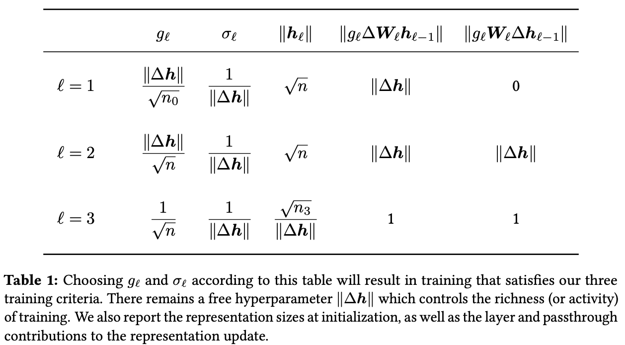
This defines the richness parameter $r$, where $||\Delta h||\sim n^r$ and $0\le r\le \frac{1}{2}$. The lower bound for $r$ comes from equation (3) while the upper bound is a reasonable heuristic. Theoretically and empirically, setting $r>\frac{1}{2}$ results in unstable training due to gradient instability.

disclaimer: this note was mostly transcribed by Gemini