Batch Norm

Batch normalization attempts to tackle the problem in neural net training of having to use low learning rates, careful parameter initialization, and not being able to use saturating nonlinearities. The authors of the original paper assert that the reason for these issues is that “the distribution of each layer’s inputs changes during training, as the parameters of the previous layers change.” To solve this fundamental problem of “internal covariate shift,” they propose batch normalization.

All the quotations from the Covariate Shift and Batch Normalization sections are from the original batch normalization paper: Batch Normalization: Accelerating Deep Network Training by Reducing Internal Covariate Shift.

Covariate Shift

Most deep learning models utilize stochastic gradient descent (SGD) with mini-batches. The authors present a common issue with it.

While stochastic gradient is simple and effective, it requires careful tuning of the model hyper-parameters, specifically the learning rate used in optimization, as well as the initial values for the model parameters. The training is complicated by the fact that the inputs to each layer are affected by the parameters of all preceding layers – so that small changes to the network parameters amplify as the network becomes deeper.

The change in the distributions of layers’ inputs presents a problem because the layers need to continuously adapt to the new distribution. When the input distribution to a learning system changes, it is said to experience covariate shift (Shimodaira, 2000). This is typically handled via domain adaptation (Jiang, 2008). However, the notion of covariate shift can be extended beyond the learning system as a whole, to apply to its parts, such as a sub-network or a layer.

The authors first assert that the consistency of the input distribution is positively correlated with the efficiency of the training process. And based off this premise, they assert that the consistency of every other layer would also correlate with more efficient training, i.e. internal covariate shift negatively correlates with efficiency. Here, consistency means consistency among examples and batches, i.e. different training or test examples look similar.

More recent work suggests that internal covariate shift is actually not a significant problem for training neural nets. However, it remains true that batch normalization significantly improves training. More on this in the “Why Does it Work?” section.

Batch Normalization

By reducing internal covariate shift through batch normalization, the authors hope to make the training process more efficient.

Batch Normalization also has a beneficial effect on the gradient flow through the network, by reducing the dependence of gradients on the scale of the parameters or of their initial values. This allows us to use much higher learning rates without the risk of divergence. Furthermore, batch normalization regularizes the model and reduces the need for Dropout (Srivastava et al., 2014)

The authors also talk about batch normalization allowing for more incautious use of saturating nonlinearities (activation functions). However, this isn’t really relevant anymore as the use of ReLU has become much more prevalent.

The authors take inspiration from attempts to reduce covariate shift in input data through whitening, i.e. linearly transforming to have zero mean, unit variance, and decorrelating. However, they argue that this isn’t feasible for other layers because

1. Repeatedly calculating the covariance matrix of all activations and its inverse square root is computationally expensive to perform at every training step.
2. The training optimization (gradient descent) does not inherently account for the whitening transformation. If you whiten the layer inputs as a separate step, the gradient updates might work against the normalization.
3. The full whitening process is not always differentiable, which poses a significant problem for training.

Thus, the authors make two “necessary simplifications.”

The first is that instead of whitening the features in layer inputs and outputs jointly, we will normalize each scalar feature independently, by making it have the mean of zero and the variance of 1. For a layer with d-dimensional input $x=(x^{(1)}...x^{(d)})$, we will normalize each dimension ${\hat{x}}^{(k)}=\frac{x^{(k)}-E[x^{(k)}]}{\sqrt{Var[x^{(k)}]}}$where the expectation and variance are computed over the training data set. As shown in (LeCun et al., 1998b), such normalization speeds up convergence, even when the features are not decorrelated.

The authors also note that forcing a certain distribution onto the model could hurt learning.

To address this, we make sure that the transformation inserted in the network can represent the identity transform. To accomplish this, we introduce, for each activation $x^{(k)}$ , a pair of parameters ${\gamma }^{(k)},{\beta }^{(k)}$, which scale and shift the normalized value: $y^{(k)}={\gamma }^{(k)}{\hat{x}}^{(k)}+{\beta }^{(k)}.$These parameters are learned along with the original model parameters, and restore the representation power of the network. Indeed, by setting ${\gamma }^{(k)}=Var[x^{(k)}]$ and ${\beta }^{(k)}=E[x^{(k)}]$, we could recover the original activations, if that were the optimal thing to do.

By doing this, the authors allow the model to learn the optimal distribution for their inputs.

Thus, the first simplification was to consider “each scalar feature independently.” Now, the authors make another simplification.

Therefore we make the second simplification: since we use mini-batches in stochastic gradient training, each mini-batch produces estimates of the mean and variance of each activation. This way, the statistics used for normalization can fully participate in the gradient backpropagation.

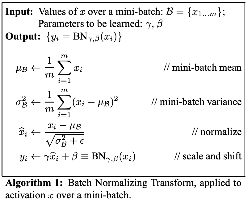
Finally, the batch normalization is presented:

Consider a mini-batch $\mathcal{B}$ of size $m$. Since the normalization is applied to each activation independently, let us focus on a particular activation $x^{(k)}$ and omit $k$ for clarity. We have $m$ values of this activation in the mini-batch, $\mathcal{B}=\{x_{\mathrm{1...}m}\}.$Let the normalized values be ${\hat{x}}_{\mathrm{1...}m}$, and their linear transformations be $y_{\mathrm{1...}m}$. We refer to the transform $B{N}_{\gamma ,\beta }:x_{\mathrm{1...}m}\to y_{\mathrm{1...}m}$as the Batch Normalizing Transform. We present the $BN$ Transform in Algorithm 1. In the algorithm, $ϵ$ is a constant added to the mini-batch variance for numerical stability.

Each normalized activation $x^{(k)}$ can be viewed as an input to a sub-network composed of the linear transform $y^{(k)}={\gamma }^{(k)}{\hat{x}}^{(k)}+{\beta }^{(k)}$, followed by the other processing done by the original network. These sub-network inputs all have fixed means and variances, and although the joint distribution of these normalized $x^{(k)}$ can change over the course of training, we expect that the introduction of normalized inputs accelerates the training of the sub-network and, consequently, the network as a whole.

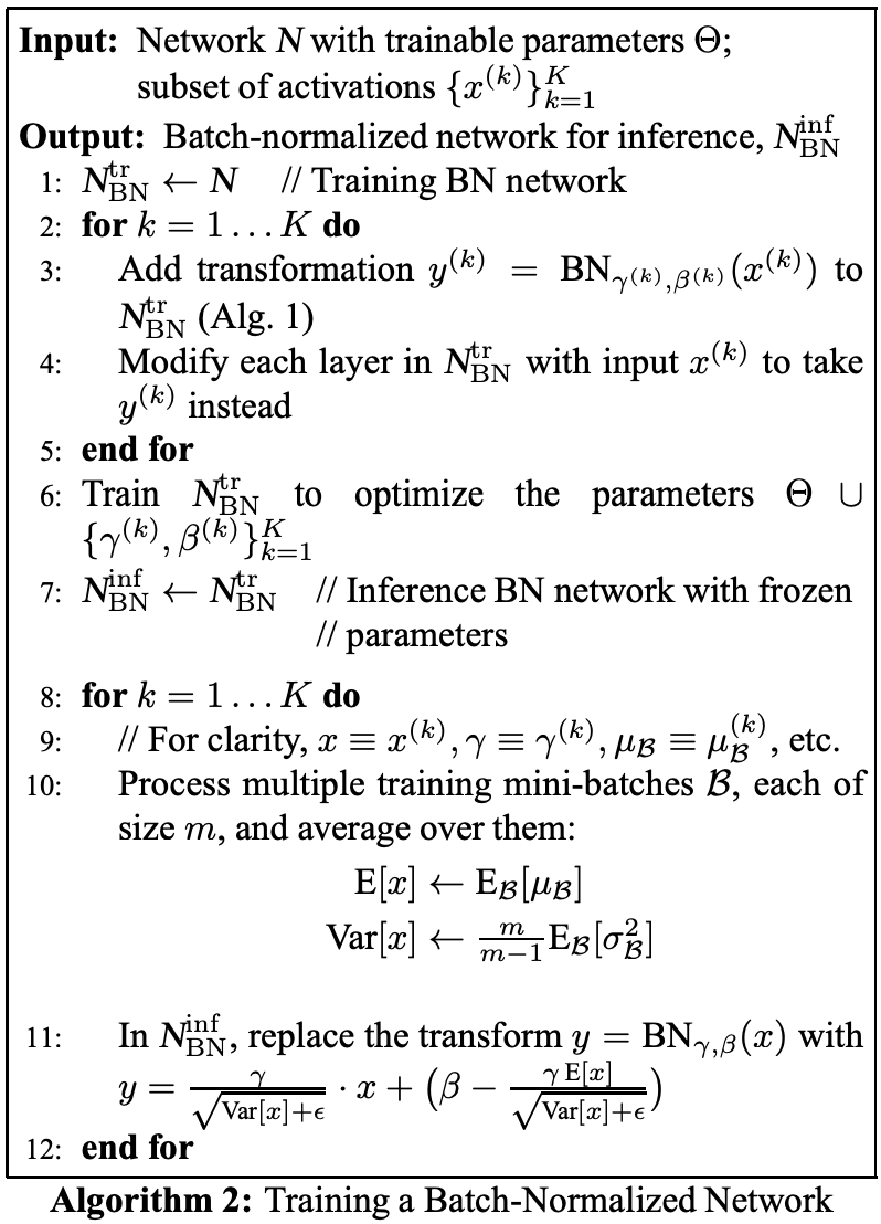
For inference, the normalization with respect to mini-batch is unnecessary. So, the authors suggest a simpler whitening procedure for inference.

Algorithm 2 summarizes the procedure for training batch-normalized networks.

Why Does it Work?

The following is from another paper examining batch normalization titled Batch Normalization Provably Avoids Rank Collapse for Randomly Initialised Deep Networks.

The difficulty of training randomly initialized, un-normalized deep networks with gradient methods is a long-known fact, that is commonly attributed to the so-called vanishing gradient effect, i.e., a decreasing gradient norm as the networks grow in depth (see, e.g., [27]). A more recent line of research tries to explain this effect by the condition number of the input-output Jacobian (see, e.g., [32, 33, 23, 7]). Here, we study the spectral properties of the above introduced initialization with a particular focus on the rank of the hidden layer activations over a batch of samples. The question at hand is whether or not the network preserves a diverse data representation which is necessary to disentangle the input in the final classification layer.

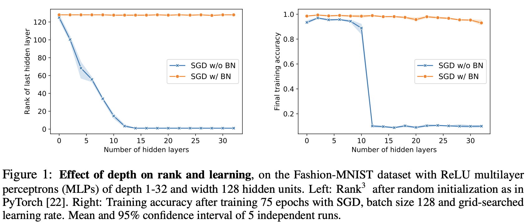
As a motivation, consider the results of Fig. 1, which plots accuracy and output rank when training batch-normalized and un-normalized neural networks of growing depth on the Fashion-MNIST dataset [31]. As can be seen, the rank in the last hidden layer of the vanilla networks collapses with depth and they are essentially unable to learn (in a limited number of epochs) as soon as the number of layers is above 10. The rank collapse indicates that the direction of the output vector has become independent of the actual input. In other words, the randomly initialized network no longer preserves information about the input. Batch-normalized networks, however, preserve a high rank across all network sizes and their training accuracy drops only very mildly as the networks reach depth 32.

The above example shows that both rank and optimization of even moderately-sized, unnormalized networks scale poorly with depth. Batch-normalization, however, stabilizes the rank in this setting and the obvious question is whether this effect is just a slow-down or even simply a numerical phenomenon, or whether it actually generalizes to networks of infinite depth.

Essentially, it seems to be that batch normalization allows for “deep information propagation.” In other words, it allows for networks to be much deeper without layers collapsing and destroying information.

If the hidden representation at the last hidden layer becomes rank one, the normalized gradients of the loss with respect to the weights in the final classification layer become collinear for any two different data points. This would mean that the gradient direction (update direction) becomes independent from the input, i.e. highly constrained and not adaptable to the inputs. A slightly weaker version of this problem would also occur if the last hidden layer simply has a (very) low rank. Then every input would be squished into a low-dimensional subspace, losing information.

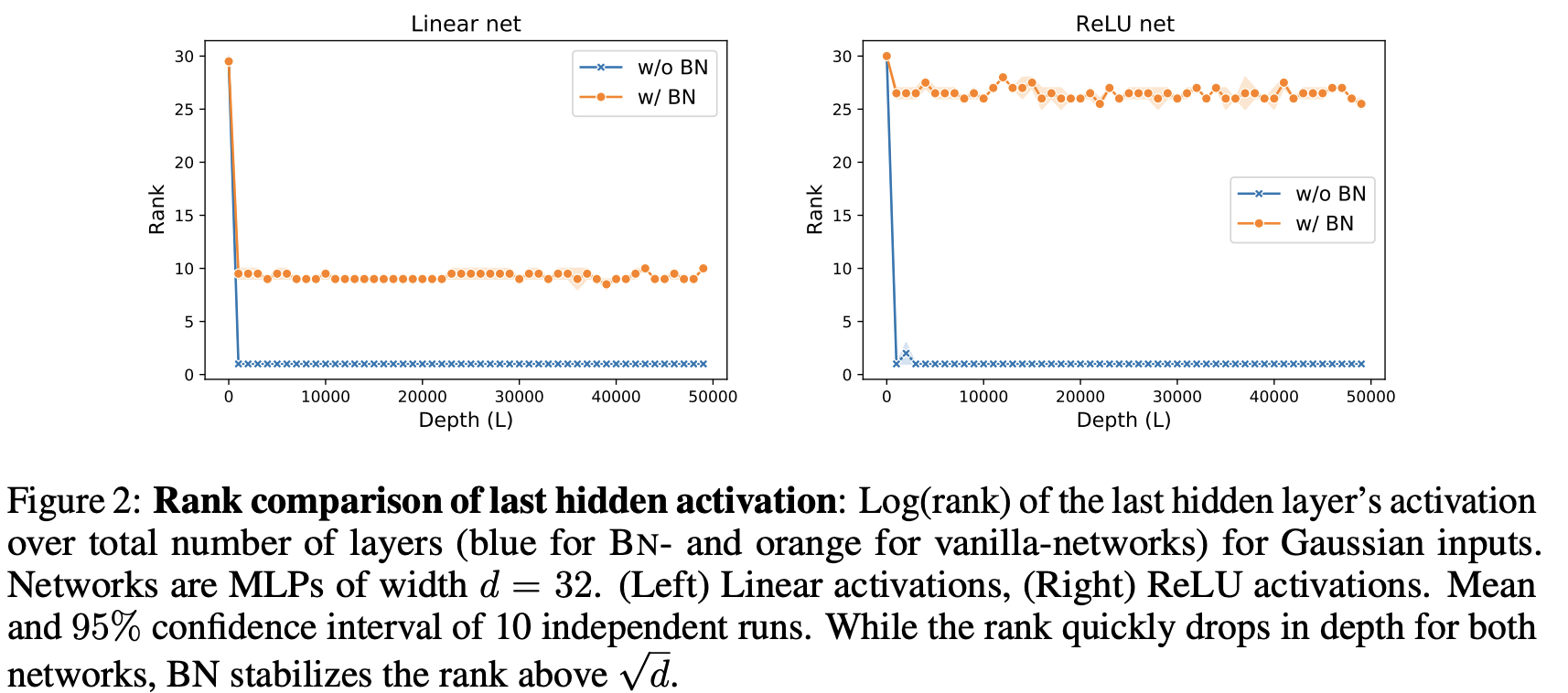
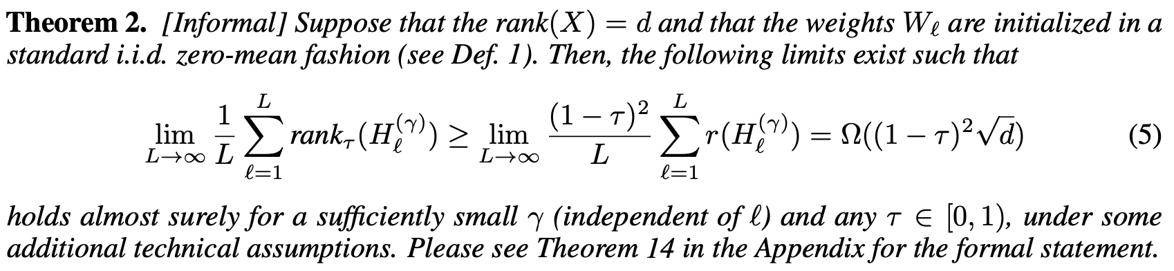
Ideally, from an information propagation perspective, the network should be able to differentiate between individual samples, regardless of its depth [27]. However, as can be seen in Fig. 2, the hidden representation of $X$ [input matrix] collapses to a rank one matrix in vanilla networks, thus mapping all $x_i$ to the same line in ${\mathbb{R}}^d$. Hence, the hidden layer activations and along with it the individual gradient directions become independent from the input $x_i$ as depth goes to infinity. We call this effect “directional” gradient vanishing (see Section 3 for a more thorough explanation). Interestingly this effect does not happen in batch-normalized networks, which yield – as we shall prove in Theorem 2 – a stable rank for any depth, thereby preserving a disentangled representation of the input and hence allowing the training of very deep networks. These results substantiate earlier empirical observations made by [7] for random BN-nets, and also validates the claim that BN helps with deep information propagation [27].

Theorem 2 shows that given a full rank input and a standard initialization scheme, the average rank of all the hidden layers in a network with batch normalization is lower-bounded by a value proportional to the square root of the network’s width. Thus, batch normalization allows the rank to not collapse given sufficient network width.

Practical Usage

The authors in the original paper suggest some further improvements to batch normalized networks:

• Increase learning rate
• Remove Dropout
• Reduce the L2 weight regularization
• Accelerate the learning rate decay
• Remove Local Response Normalization
• Shuffle training examples more thoroughly
• Reduce the photometric distortions

References: Batch Normalization: Accelerating Deep Network Training by Reducing Internal Covariate Shift Batch Normalization Provably Avoids Rank Collapse for Randomly Initialised Deep Networks

Resources: PyTorch BatchNorm1d Towards Training Without Depth Limits: Batch Normalization Without Gradient Explosion