Self-Explaining Neural Networks

The authors propose an ante-hoc explainability framework for training neural networks that are inherently interpretable. Evaluating based on explicitness, faithfulness, and stability, the authors show that existing methods for explainability are unsatisfactory. They propose SENNs and show that they are superior with respect to the aforementioned criteria.

From Linear Models to SENNs

The main intuition is that linear models are highly interpretable as we can see exactly what features the model is placing emphasis on, and they make consistent predictions based on a small number of parameters.

For input features $x_1,...,x_n\in \mathbb{R}$, and associated parameters ${\theta }_1,...,{\theta }_n\in \mathbb{R}$ the linear regression model is given by $f(x)={\sum }_i^n{\theta }_i{x}_i+{\theta }_0$. This model is arguably interpretable for three specific reasons: i) input features ($x_i$’s) are clearly anchored with the available observations, e.g., arising from empirical measurements; ii) each parameter ${\theta }_i$ provides a quantitative positive/negative contribution of the corresponding feature $x_i$ to the predicted value; and iii) the aggregation of feature specific terms ${\theta }_i{x}_i$ is additive without conflating feature-by-feature interpretation of impact.

The authors aim to generalize this kind of linear model to simultaneously enrich its learning capabilities while maintaining its interpretability. The generalization is achieved in 3 steps:

1. Generalizing coefficients
2. Utilizing rich feature bases
3. Generalizing aggregation function.

Generalizing Coefficients

The idea is to have the coefficients depend on the input $x$, i.e. have the coefficients $\theta$ be functions with respect to $x$.

Specifically, we define (offset function omitted) $f(x)=\theta (x{)}^{T}x$, and choose $\theta$ from a complex model class $\theta$, realized for example via deep neural networks.

Crucially, with just this generalization of $\theta$, the model becomes “as powerful as any deep neural network” since $\theta$ could simply be a neural network. However, by doing so, we reintroduce black box neural nets and lose the interpretability that we had in scalar parameters. Thus, the authors assert that we must enforce “close” inputs $x$ and $x^{\prime }$ to have similar parameter values $\theta (x)$ and $\theta (x^{\prime })$.

More precisely, we can, for example, regularize the model in such a manner that ${\nabla }_{x}f(x)\approx \theta (x_0)$ for all $x$ in a neighborhood of $x_0$. In other words, ==the model acts locally, around each $x_0$, as a linear model with a vector of stable coefficients $\theta (x_0)$==. The individual values $\theta (x_0{)}_i$ act as and are interpretable as coefficients of a linear model with respect to the final prediction, but adapt dynamically to the input, albeit varying slower than x.

Feature Basis

Typical interpretable models tend to consider each variable (one feature or one pixel) as the fundamental unit which explanations consist of. However, pixels are rarely the basic units used in human image understanding; instead, we would rely on strokes and other higher order features. We refer to these more general features as interpretable basis concepts and use them in place of raw inputs in our models.

We define a function $h(x):\mathcal{X}\to featurespace$ that takes raw input features and projects them into a more interpretable feature space. The authors offer several suggestions for $h$:

we consider functions $h(x):\mathcal{X}\to \mathcal{Z}\subset {\mathbb{R}}^k$, where $\mathcal{Z}$ is some space of interpretable atoms. Naturally, $k$ should be small so as to keep the explanations easily digestible. Alternatives for $h(\cdot )$ include: (i) subset aggregates of the input (e.g., with $h(x)=Ax$ for a boolean mask matrix $A$), (ii) predefined, pre-grounded feature extractors designed with expert knowledge (e.g., filters for image processing), (iii) prototype based concepts, e.g. $h_i(x)=||x-z_i||$ for some $z_i\in \mathcal{X}$ [12], or learnt representations with specific constraints to ensure grounding [19]. Naturally, we can let $h(x)=x$ to recover raw-input explanations if desired.

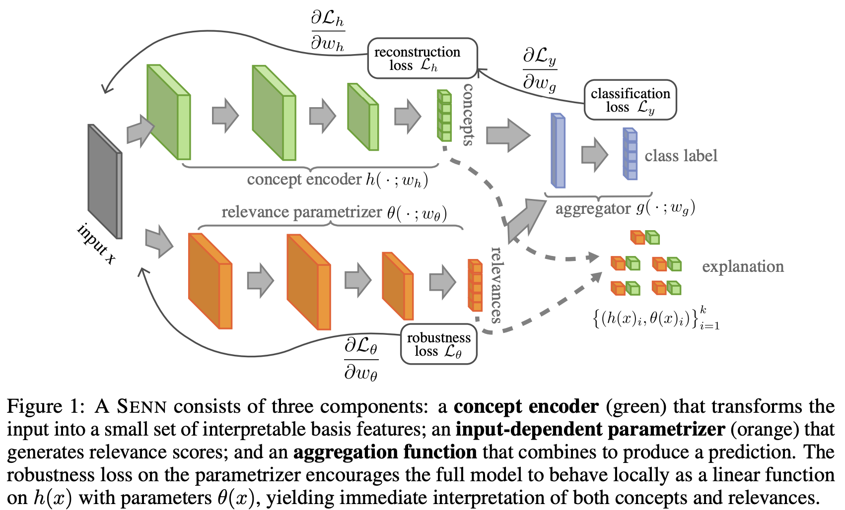
With the generalized coefficients and the feature basis, we have the following model: $f(x)=\theta (x{)}^{T}h(x)={\sum }_{i=1}^K\theta (x{)}_{i}h(x{)}_i.$

Since each $h(x{)}_i$ remains a scalar, it can still be interpreted as the degree to which a particular feature is present. In turn, with constraints similar to those discussed above $\theta (x{)}_i$ remains interpretable as a local coefficient. Note that the notion of locality must now take into account how the concepts rather than inputs vary since the model is interpreted as being linear in the concepts rather than $x$.

Generalized Aggregation

The last step is to generalize the summation present in $f$. We can consider more generally, any function $g(z_1,...,z_k)$ that effectively aggregates the $\theta (x{)}_{i}h(x{)}_i$‘s.

Naturally, in order for this function to preserve the desired interpretation of $\theta (x)$ in relation to $h(x)$, it should: i) be permutation invariant, so as to eliminate higher order uninterpretable effects caused by the relative position of the arguments, (ii) isolate the effect of individual $h(x{)}_i$‘s in the output (e.g., avoiding multiplicative interactions between them), and (iii) preserve the sign and relative magnitude of the impact of the relevance values $\theta (x{)}_i$ .

Self Explaining Models

The authors use the following definition to enforce the notion of “local stability.”

Definition 3.2. $f:\mathcal{X}\subseteq {\mathbb{R}}^n\to {\mathbb{R}}^m$ is locally difference bounded by $h:\mathcal{X}\subseteq {\mathbb{R}}^n\to {\mathbb{R}}^k$ if for every $x_0$ there exist $\delta >0$ and $L\in \mathbb{R}$ such that $||x-x_0||<\delta$ implies $||f(x)-f(x_0)||\le L||h(x)-h(x_0)||$.

The following definition defines the class of functions the authors constitute as self-explaining prediction models:

Definition 3.3. Let $x\in \mathcal{X}\subset {\mathbb{R}}^n$ and $\mathcal{Y}\subseteq {\mathbb{R}}^m$ be the input and output spaces. We say that $f:\mathcal{X}\to \mathcal{Y}$ is a self-explaining prediction model if it has the form $f(x)=g({\theta }_1(x)h_1(x),...,{\theta }_k(x)h_k(x))$ where:

• P1) $g$ is monotone and completely additively separable
• P2) For every $z_i:={\theta }_i(x)h_i(x)$, $g$ satisfies $\frac{\partial g}{\partial z_i}\ge 0$
• P3) $\theta$ is locally difference bounded by $h$
• P4) $h_i(x)$ is an interpretable representation of $x$
• P5) $k$ is small. In that case, for a given input $x$, we define the explanation of $f(x)$ to be the set ${\mathcal{E}}_f(x)\equiv {(h_i(x),{\theta }_i(x))}_{i=1}^k$ of basis concepts and their influence scores.

Since our aim is maintaining model richness even in the case where the $h_i$ are chosen to be trivial input feature indicators, we rely predominantly on $\theta$ for modeling capacity, realizing it with larger, higher-capacity architectures.

The tricky part about enforcing P3 is that we want the model to be linear in terms of the concepts, not $x$, i.e. we want $f$ to be stable with respect to $h$.

For this, let us consider what $f$ would look like if the ${\theta }_i$’s were indeed (constant) parameters. Looking at $f$ as a function of $h(x)$, i.e. $f(x)=g(h(x))$, let $z=h(x)$. Using the chain rule we get ${\nabla }_{x}f={\nabla }_{z}f\cdot J_x^h$ , where $J_x^h$ denotes the Jacobian of $h$ (with respect to $x$). At a given point $x_0$, we want $\theta (x_0)$ to behave as the derivative of $f$ with respect to the concept vector $h(x)$ around $x_0$, i.e., we seek $\theta (x_0)\approx {\nabla }_{z}f$. Since this is hard to enforce directly, we can instead plug this ansatz in ${\nabla }_{x}f={\nabla }_{z}f\cdot J_x^h$ to obtain a proxy condition: ${\mathcal{L}}_{\theta }(f(x)):=||{\nabla }_{x}f(x)-\theta (x{)}^T{J}_x^h(x)||\approx 0$ All three terms in ${\mathcal{L}}_{\theta }(f)$ can be computed, and when using differentiable architectures $h(\cdot )$ and $\theta (\cdot )$, we obtain gradients with respect to (3) [above equation] through automatic differentiation and thus use it as a regularization term in the optimization objective. With this, we obtain a gradient-regularized objective of the form ${\mathcal{L}}_y(f(x),y)+\lambda {\mathcal{L}}_{\theta }(f)$, where the first term is a classification loss and $\theta$ a parameter that trades off performance against stability—and therefore, interpretability— of $\theta (x)$.

This is so incredibly clever I’m at a loss for words. Essentially, we know we want $a\approx b$ to be true. We also know that $x=b\cdot c$. Since it’s difficult to directly encode the $a\approx b$ objective into the loss function, we instead encode $x\approx a\cdot c$ into the loss function. A very nice problem-solving technique seen used in the wild!

Learning Interpretable Basis Concepts

Basis concepts which serve as “units” of explanation are ideally “expert-informed.” However, in cases where expert knowledge is scarce or expensive, such concepts can be learned. The authors propose the following desiderata for interpretable concepts:

(i) Fidelity: the representation of $x$ in terms of concepts should preserve relevant information, (ii) Diversity: inputs should be representable with few non-overlapping concepts, and (iii) Grounding: concepts should have an immediate human-understandable interpretation.

The authors then describe how they achieved their proposed desiderata:

Here, we enforce these conditions upon the concepts learnt by SENN by: (i) training h as an autoencoder, (ii) enforcing diversity through sparsity and (iii) providing interpretation on the concepts by prototyping (e.g., by providing a small set of training examples that maximally activate each concept). Learning of h is done end-to-end in conjunction with the rest of the model. If we denote by $h_{dec}(\cdot ):{\mathbb{R}}^k\to {\mathbb{R}}^n$ the decoder associated with $h$, and $\hat{x}:=h_{dec}(h(x))$ the reconstruction of $x$, we use an additional penalty ${\mathcal{L}}_h(x,\hat{x})$ on the objective, yielding the loss: ${\mathcal{L}}_y(f(x),y)+\lambda {\mathcal{L}}_{\theta }(f)+\xi {\mathcal{L}}_h(x,\hat{x})$Achieving (iii), i.e., the grounding of $h(x)$, is more subjective. A simple approach consists of representing each concept by the elements in a sample of data that maximize their value, that is, we can represent concept $i$ through the set $X^i=argma{x}_{\hat{X}\subseteq X,|\hat{X}|=l}{\sum }_{x\in \hat{X}}h(x{)}_i$ where $l$ is small. Similarly, one could construct (by optimizing $h$) synthetic inputs that maximally activate each concept (and do not activate others), i.e., $argma{x}_{x\in X}{h}_i(x)-{\sum }_{j\ne i}{h}_j(x)$. Alternatively, when available, one might want to represent concepts via their learnt weights—e.g., by looking at the filters associated with each concept in a CNN-based $h(\cdot )$. In our experiments, we use the first of these approaches (i.e., using maximally activated prototypes), leaving exploration of the other two for future work.

References: Towards Robust Interpretability with Self-Explaining Neural Networks