This looks like That

This paper concretely implements the ideas of interpretability discussed in Jaakkola et al, Towards Robust Interpretability with Self-Explaining Neural Networks. Although, it is worth noting that the notion of interpretability is more loosely defined. The authors lean more toward accuracy in the interpretability-accuracy tradeoff. This perspective is elaborated in Elton, Self-explaining AI as an alternative to interpretable AI.

Motivation

The key intuition comes from the way humans reason about images. The authors note that

When we are faced with challenging image classification tasks, we often explain our reasoning by dissecting the image, and pointing out prototypical aspects of one class or another. The mounting evidence for each of the classes helps us make our final decision.

ProtoPNet identifies parts of an image where it thinks this looks like that prototypical part of some class and it “makes its prediction based on a weighted combination of the similarity scores between parts of the image and the learned prototypes.” The model is interpretable in the sense that it has a “transparent reasoning process when making predictions.”

ProtoPNet

Architecture

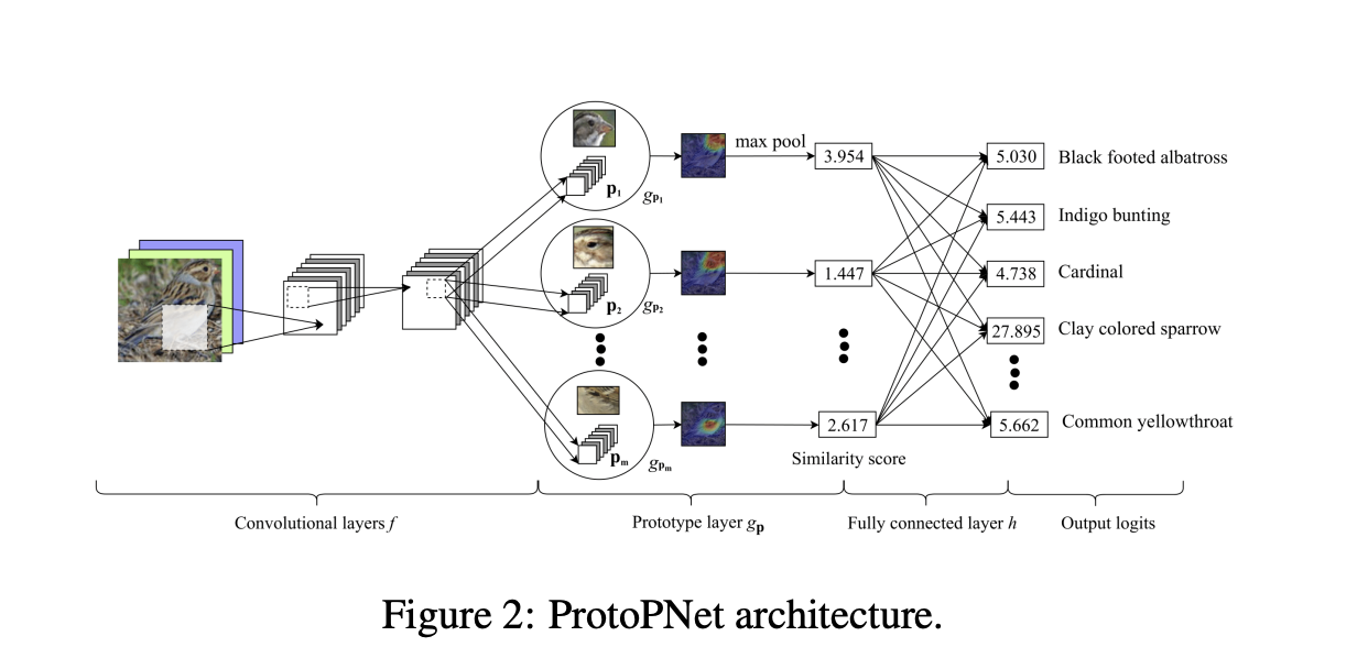The first part of the model, the convolutional layers, outputs a latent representation $f(x)$ of the input image $x$. During the training process the model learns $m$ prototypes $\mathbf{P}=\{{\mathbf{p}}_{\mathbf{j}}{\}}_{\mathbf{j}=1}^{\mathbf{m}}$ which all have the same depth as any given $f(x)$ but different height and width.

Since the depth of each prototype is the same as that of the convolutional output but the height and the width of each prototype is smaller than those of the whole convolutional output, each prototype will be used to represent some prototypical activation pattern in a patch of the convolutional output, which in turn will correspond to some prototypical image patch in the original pixel space.

In the prototype layer $g_{\mathbf{P}}$, for every prototype $p_j$, the squared $L^2$ distances between $p_j$ and all patches of $f(x)$ with the same shape are calculated, and inverted to form similarity scores.

The result is an activation map of similarity scores whose value indicates how strong a prototypical part is present in the image. This activation map preserves the spatial relation of the convolutional output, and can be upsampled to the size of the input image to produce a heat map that identifies which part of the input image is most similar to the learned prototype. The activation map of similarity scores produced by each prototype unit $g_{p_j}$ is then reduced using global max pooling to a single similarity score, which can be understood as how strongly a prototypical part is present in some patch of the input image.

Lastly, the fully connected layer $h$ takes the similarity scores and uses a softmax to yield predicted probabilities for each class.

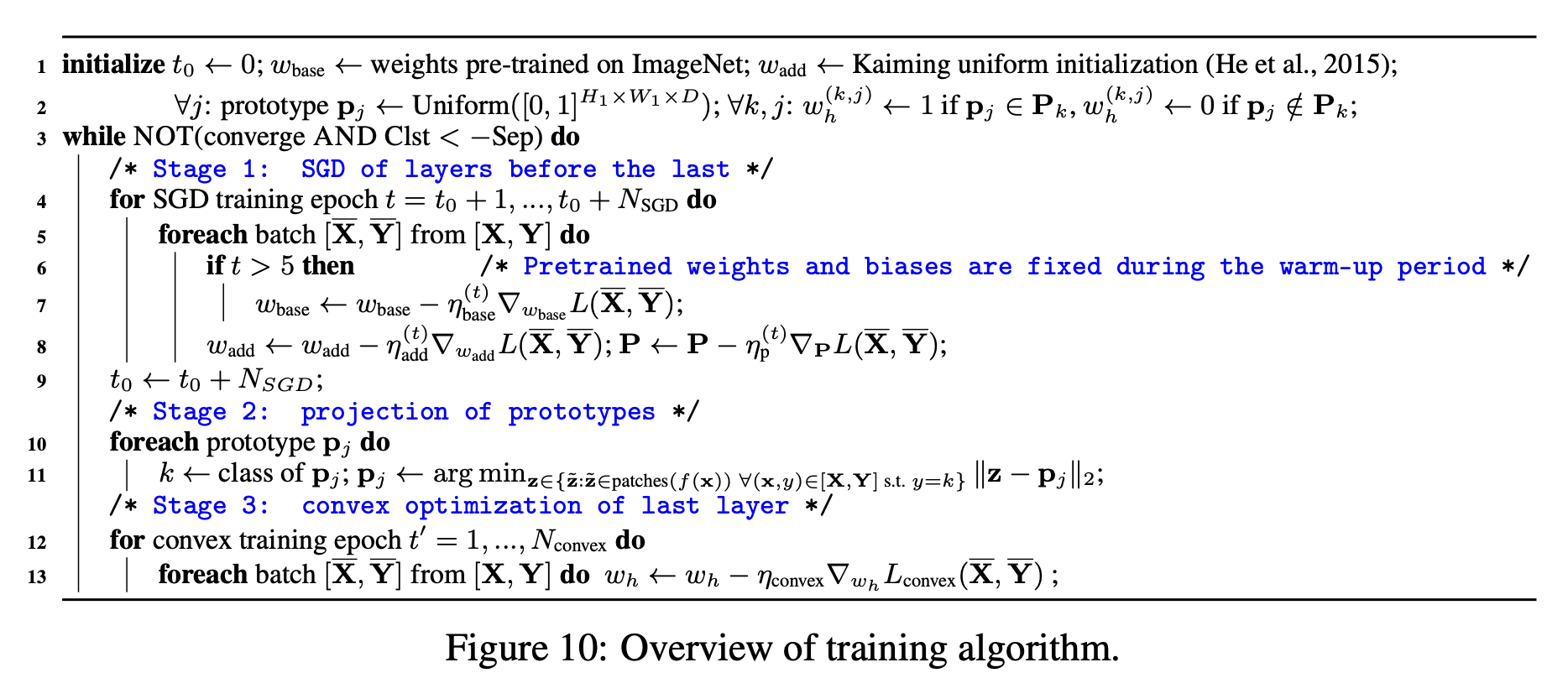
Training

The first stage is essentially a fancy clustering algorithm.

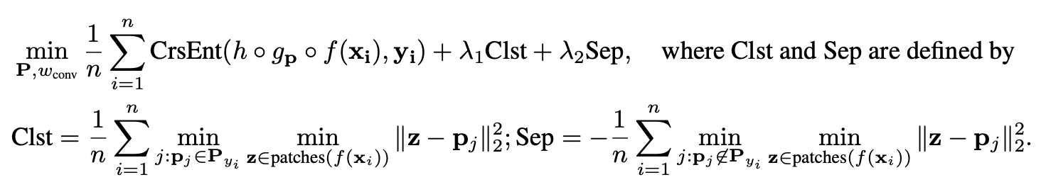
In the first training stage, we aim to learn a meaningful latent space, where the most important patches for classifying images are clustered (in $L^2$-distance) around semantically similar prototypes of the images’ true classes, and the clusters that are centered at prototypes from different classes are well-separated. To achieve this goal, we jointly optimize the convolutional layers’ parameters $w_{conv}$ and the prototypes $\mathbf{P}=\{{\mathbf{p}}_{\mathbf{j}}{\}}_{\mathbf{j}=1}^{\mathbf{m}}$ in the prototype layer $g_{\mathbf{P}}$ using SGD, while keeping the last layer weight matrix $w_h$ fixed.

The second stage is the key part in implementing the following constraint:

we propose to constrain each convolutional filter to be identical to some latent training patch. This added constraint allows us to interpret the convolutional filters as visualizable prototypical image parts and also necessitates a novel training procedure.

The authors accomplish this by projecting “each prototype $p_j$ onto the nearest latent training patch from the same class as that of $p_j$.”

Mathematically, for prototype $p_j$ of class $k$, i.e., $p_j\in {\mathbf{P}}_{\mathbf{k}}$, we perform the following update: $p_j\leftarrow argmi{n}_{\mathbf{z}\in {\mathcal{Z}}_{\mathbf{j}}}||\mathbf{z}-{\mathbf{p}}_{\mathbf{j}}|{|}_2,\text{mbox}where{\mathcal{Z}}_j=\{\tilde{z}:\tilde{z}\in \text{mbox}patches(f(x_i))\forall i\text{mbox}s.t.y_i=k\}.$

The third stage is a convex optimization of the feedforward weight matrix. The convolutional layer and prototype layer stay fixed, thus keeping the latent representations constant.

Probabilistic Interpretation

The authors show in the supplementary material that ProtoPNet is essentially an instantiation of the above predictive model derived from two reasonable assumptions.

The first assumption is that

for any given image $x$, the probability of $X$ being of value $x$ given all of its closest latent patches to prototypes of class $k$ and the fact that the image is indeed of class k is the same for every single class $k\in \{1,...,K\}$. We can roughly think of this assumption as: for any class, knowing an unknown image’s closest latent patches to prototypes of that class and the fact that unknown image actually belongs to that class gives us the same level of uncertainty about the true value of the image.

The first assumption is essentially an assumption about the equitable quality of prototypes, i.e. no one class has a much better set of prototypes that more easily allows identification of $x$. This would be true if every set of prototypes along with information about the class of $x$ were sufficient to reconstruct $x$ at the same fidelity no matter the class. I’m actually not so sure that this is a reasonable assumption to make. It certainly depends highly on the data one is working with.

The second assumption is that the random variables $\{f_l^k(X)\}$ are independent over the subspace $\{(z_1^k,...,z_{m_k}^k)\in {\Omega }^{m_k}:\exists x\in Xs.t.z_1^k=f_1^k(x),...,z_{m_k}^k=f_{m_k}^k(x)\}$. This, again is a naive and somewhat unreasonable assumption to make. However, it does simplify the math dramatically.

The authors assert that ProtoPNet does the following probability prediction:

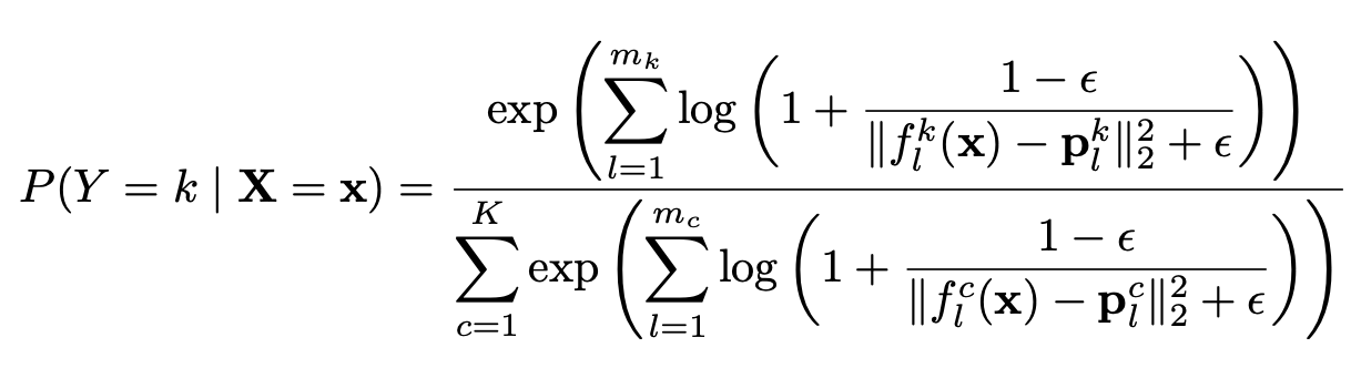
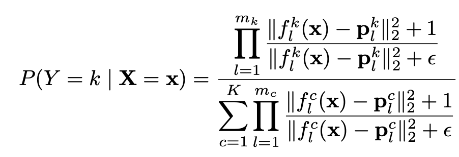
Comparing Equations (10) and (11), we see that for our current model, we have: (1) $\Omega =[0,1{]}^{H_1\times W_1\times D}$; (2) $P(Y=c)=\frac{1}{K}$, for all $c\in \{1,...,K\}$; and (3) $d_l^k(r)=C_l^k\cdot \frac{r^2+1}{r^2+ϵ}$. The constant $C_l^k$ ensures that the integration over the latent domain $\Omega$ gives value of 1. When the number of prototypes for every class is the same, the ${\prod }_{l=1}^{m_k}{C}_l^k$ will approximately cancel out in the numerator and denominator of Equation 10, leaving us with the current expression we use for our classification model.

The assumptions made earlier mean that ProtoPNet is in essence, a sophisticated but naive Bayes classifier. Perhaps this isn’t mathematically satisfying, but the results seem to back up the approach.

---

Though ProtoPNet defines interpretability more loosely than proposed in Jaakkola et al, the architecture itself is remarkably similar to the one suggested in it. The process of generating prototypes (stage 1 of training), is essentially a process of generating a suitable feature basis. Furthermore, the criteria of fidelity, diversity, and grounding are built in to the clustering algorithm used to generate the prototypes. Technically, the feature basis ProtoPNet uses is the similarity scores generated during the inference process, as that is what is fed into the fully connected linear layer. And perhaps it is a little less clear that the similarity scores satisfy fidelity, diversity, and grounding. Nevertheless, the last fully connected layer is a linear model, and in fact, is less general than the one described Jaakkola et al as the relevance scores (weights) for each similarity score is a fixed number for all inputs.

The biggest difference between ProtoPNet and the architecture proposed in Jaakkola et al is that in ProtoPNet, most of the modeling capacity is in the feature bases. The relevance scores, i.e. the weights of the fully connected layer, are fixed for all inputs while the feature basis, i.e. the similarity scores between the input and the prototypes, is a complex, high-capacity ConvNet architecture. It seems that Jaakkola et al opted to shift complexity to the relevance scores as to keep the feature basis simple and easily interpretable. However, they still use an autoencoder to develop their feature basis, so it really cannot be said that their version was substantially more interpretable.

References:

• This Looks Like That: Deep Learning for Interpretable Image Recognition
• This Looks Like That: Deep Learning for Interpretable Image Recognition (Supplementary Material)
• Towards Robust Interpretability with Self-Explaining Neural Networks
• Self-explaining AI as an alternative to interpretable AI